Monte Carlo Localization for VEX teams

in this post, I describe an implementation of Monte Carlo Localization (MCL) for VEX V5 Robotics Competition teams. I’ll explain when a team will need MCL, how it works, and how it looks as code. before we continue, I need to make a very important disclaimer.

DO NOT USE MY CODE! this isn’t just because it is illegal to copy someone’s code, but also because my code is not suitable for competition use. I explain a lot of my code’s footguns in the explanation below.

this is not the implementation we use in the VEX AI team 3151A, which is GPU-accelerated and has other optimizations, but this captures the majority of the important logic.

general terminology

Localization is just figuring out where your robot is on the field. this generally involves determining or estimating your pose (position and orientation), generally expressed as $(x, y, \theta)$.

Displacement or delta is the change in pose, generally expressed as $(\Delta x, \Delta y, \Delta \theta)$.

why you might need MCL

most VEX teams use odometry (with tracking wheels and/or an inertial movement unit) sensors to localize their robot.

however, odometry has a big issue. it is “dead-reckoning” — in other words, it is calculating displacement over a short time interval and adding it up (numerically integrating). this is great for 15-second auton runs, but for 1-minute skills, it quickly becomes inaccurate. inherent error in sensors and displacement calculations compound over time.

the solution is to add two things to your localization system:

1. an absolute sensor, which you can compare against your pose. the key feature of this sensor is that its value is not dependent on previous states/poses. in VEX this is typically a distance sensor, which returns the distance to the nearest field wall (or an obstacle).

however, using an absolute sensor by itself is not enough. if your distance sensor is obstructed, voila! — your robot now thinks it has teleported backwards. this is where another algorithm comes in.

2. a filter algorithm, which combines the absolute sensor with the odometry to get a more accurate pose. this is where MCL comes in.

how MCL works

particle filters

generally these filter algorithms are designed to be Bayesian — in simple terms, they estimate the pose as a distribution. it is almost naive to represent robot pose with a single state because that means we are 100% certain in that prediction (which is never true). in other words, the distribution is spread out to account for uncertainty in our pose. think this:

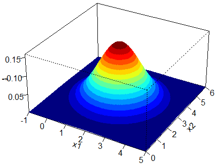
(obviously, this would have to be in 4D to account for theta but shhhh)

the height of each point represents the probability of the robot being at that pose. this is a probability distribution.

MCL basically “cheats” a little bit. instead of storing the distribution (which is a lot of math), it stores a bunch of particles. imagine each particle as a point in the above distribution. each particle is just a pose. note that we don’t actually know the distribution (and the distribution is constantly changing) — we have a bunch of particles, and we try to make them represent the current distribution as closely as possible.

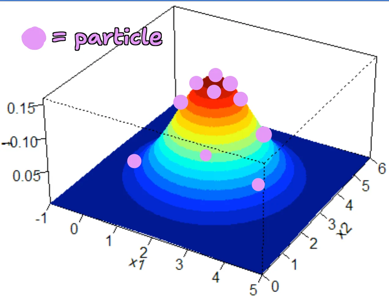
this is what a good MCL distribution should look like. note that there are more particles on the higher areas (the areas that are more likely to be correct), which is what you’d expect if you randomly sampled that distribution.

this is true for particle filters in general (MCL is a particle filter). other algorithms like Kalman filters also estimate a distribution but in a different form.

the key idea of MCL is to combine a dead-reckoning and absolute sensor system, by using the dead-reckoning system to update particles, but also “weighting” the particles based on the absolute sensor system and using that to remove lower-weighted particles + keep higher-weighted particles.

think of it as natural selection for particles.

algorithm overview

now let’s go through the basic steps of running MCL and explaining why they each make sense.

throughout, I will explain what the theory expects you to do (i.e., what is the natural consequence of the math) and what I do in my implementation (which is generally jankier but often more performant).

setup

1. initialize particles. in VEX you probably know approximately where your robot starts. this means you thus want to initialize your particles around that point.
   • in theory: initialize particles randomly around the starting point, with a normal distribution to account for uncertainty in setup.
   • in practice: initialize all particles at the starting point. saves computation and the particles will naturally spread out in a later step.
2. define your weighting function. basically, the goal of this function is to return the height of a given pose (see above distribution picture) — i.e., estimate the probability of the robot being at that pose, given the value of an absolute sensor (the weight is often not directly the same as probability, but heavily related). this is one of the most important functions you will write.

   • in theory:

     1. use distance sensor offsets (which you define somewhere) to figure out where the distance sensor would be mounted, and in what orientation, if that pose is correct.
     2. raycast from the distance sensor to the field walls to calculate what the expected distance of the distance sensor is, if that pose is correct.
     3. compare the expected distance to the actual distance, and return a probability based on that. the probability should be 0% if the error is above a certain threshold (to decrease perturbations from outliers or obstacles).
     4. multiply probabilites across scans.

   • in practice:

     • I don’t use distance sensor offsets for simplicity, and pretend that the distance sensor is at the center of the robot (obviously something you will need to change in your own implementation).
     • I then use basic trigonometry to calculate where the distance sensor’s beams should have landed (as an x/y point). finally, I compare that point to wall to get distance to the wall. this is extremely compute-efficient but relies on having a rectangular field (which V5RC does). however, on such a field, it does return the same results as raycasting. to adapt this to a non-rectangular field, you would need to use the theoretical approach above.
     • after I get distance, I return a probability based on the Gaussian distribution, which is a bell curve. this is a very common way to estimate probabilities in MCL.
     • I do this to compare every received scan beam to the particle, then sum the probabilities to get the total probability of that particle being correct.
     • I then sum the probabilities across all beams to get the total probability of that particle being correct. theory recommends using product of probabilities (and that is what the math says if you derive it) but I find summing is easier to tune.

run MCL

this part gets repeated, on a consistent basis. that can be once every 5ms, once every time to get new odom displacements, your choice. it generally gets split into two steps — update (which uses odometry) and resample (which uses the absolute sensor).

part 1. update step

3. get odometry displacements. this is what standard odometry does, you can probably copy most of the logic over from there. (I don’t include displacement calculation in my implementation because it depends on sensor configuration.) then, add that displacement to each particle’s pose, to update it with the odometry data.

4. perturb particles. generate a tiny bit of random noise (as a delta) and add it to each particle’s pose. this is to account for uncertainty in odometry and to prevent particles from clustering together. otherwise, we might end up with “overconvergence” where all particles are at the exact same pose, which is not what we want — the whole point of MCL is to account for uncertainty. (what we do want is for particles to all end up close to one another, just while maintaing some diversity.) by adding random noise, we broaden our possible guesses for what our pose is.

tuning opportunity! the amount of noise you add is a very important parameter. you’ll want separate noise values for x/y and theta, and it should be proportional to your expectations of your odometry drift. for example, if you think your inertial sensor drifts by a maximum of 5 degrees per second, and you run 50 MCL iterations per second, you should add a maximum of 5 / 50 = 0.1 degrees of noise per time step to theta.

part 2. resample step

5. weight particles. for each particle, call the weighting function to get the probability of that particle being correct. store that probability. after this step, you can imagine seeing the particles the way it is visualized in the above image, with height representing probability. however, since the particles are random, they won’t properly represent the distribution yet.

6. resample particles. this is a very important step. we want to keep the particles that are more likely to be correct, and remove the ones that are less likely to be correct. there are a lot of ways to do this. I use a version of Stochastic Universal Resampling for this. how my implementation works is pretty difficult to explain, but the general idea is that the probably of a particle being selected is proportional to its probability of being correct.

after this step, you’ll have a new set of particles that are the same size, but, after updates from odometry and distance sensors, are more likely to be correct. the distribution has thus “evolved” to be more accurate.

code walkthrough

each part of my code pretty cleanly maps to one of the steps above.

🚨WARNING🚨 if you somehow still think you can copy-and-paste my code, this is the part where you will realize it is impossible. my code is written in Python. the VEX micropython interpreter is far too slow to run efficient MCL. you will need to rewrite it in C++ or C, and I’m not planning to do it for you.

if you are trying to use MCL for something else, or on a coprocessor to the brain, you should use an efficient library such as NumPy for fast vectorized operations.

this code is a minimal modification from the code I link at the top of this article.

all distances are in inches, and angles are in radians. we use standard position for angles (the positive x-axis is 0 rad).

in general, if you see a variable with type

tuple[float, float, float]

it is a pose — that type is for a tuple of three decimal values (x, y, and theta).

math imports

if you don’t know what these functions do, either 1) read the docs or 2) make sure you understand trigonometry.

from math import cos, sin, exp, pi, sqrt, radians
from random import random # returns in [0, 1)

constants

these are the things you’ll want to tune.

N_PARTICLES = 100
GAUSSIAN_STDEV = 1
GAUSSIAN_FACTOR = 1

THETA_NOISE = radians(2)
XY_NOISE = 0.1

the GAUSSIAN_* variables are related to the Gaussian distribution used in weighting. you can use that to tune the shape of the distribution.

base classes

class Beam:
    angle: float # radians
    distance: float # inches

class Particle:
    def __init__(self, x: float = 0, y: float = 0, theta: float = 0, weight: float = -1):
        self.x = x
        self.y = y
        self.theta = theta
        self.weight = weight
    def copy(self) -> 'Particle':
        return Particle(self.x, self.y, self.theta, self.weight)
    def update_delta_noise(self, delta: tuple[float, float, float]):
        self.x += XY_NOISE * 2 * (random() - 0.5) + delta[0]
        self.y += XY_NOISE * 2 * (random() - 0.5) + delta[1]
        self.theta += THETA_NOISE * 2 * (random() - 0.5) + delta[2]

pretty self-explanatory. we initialize Particle with a sentinel value for weight of -1 to indicate it has not been weighted yet.

for update_delta_noise, we use 2 * (random() - 0.5) to convert from a random number in [0, 1) to a random number in [-1, 1). the delta parameter is a tuple of the odometry displacement.

weighting

the following are all methods implemented on the Particle class.

    def expected_point(self, beam: Beam) -> tuple[float, float, float]:
        global_theta = self.theta + beam.angle
        return (
            self.x + beam.distance * cos(global_theta),
            self.y + beam.distance * sin(global_theta),
            global_theta
        )

↑ this method basically asks, if this Particle is correct, where would this Beam land? I’m not going to go through the derivation of this equation but it is pretty easy to derive with polar coordinates

    @staticmethod
    def distance_to_wall(point: tuple[float, float, float]) -> float:
        # this approximates distance from point to wall
        # **not as accurate as raycasting**
        # but works fine in my experience
        return min([
            abs((point[0] - 72) / cos(point[2])),
            abs((point[0] + 72) / cos(point[2])),
            abs((point[1] - 72) / sin(point[2])),
            abs((point[1] + 72) / sin(point[2]))
        ])

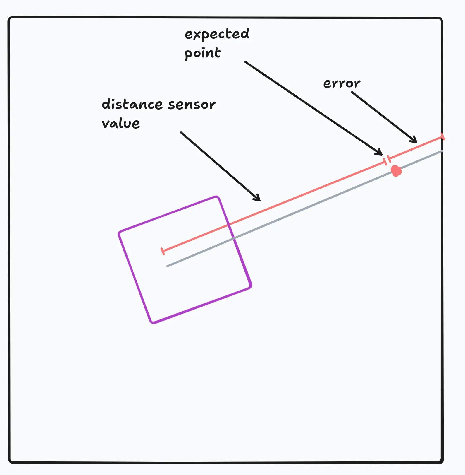
↑ this method gets the distance from a point to the wall. this returns the same value as raycasting in a simplified manner. it scales according to cosine/sine to account for the angle of the beam. the image ↓ ought to help you understand the relation between these quantities.

    @staticmethod
    def gaussian(x: float) -> float:
        return GAUSSIAN_FACTOR * exp(-0.5 * (x / GAUSSIAN_STDEV) ** 2) / (GAUSSIAN_STDEV * sqrt(2 * pi))

↑ a minimal implementation of the Gaussian distribution.

    def update_weight(self, beams: list[Beam]):
        self.weight = sum([
            self.gaussian(self.distance_to_wall(self.expected_point(beam)))
            for beam in beams
        ])

↑ exactly as discussed in the steps. we calculate the expected point for each beam, then calculate the distance to the wall, and finally use that to calculate the weight of the particle. pretty nice function nesting :D

(note that sum is a builtin Python function.)

that wraps up the Particle class.

main mcl

class MCL:
    def __init__(self):
        self.particles = [Particle() for _ in range(N_PARTICLES)]
        self.average_pose = (0, 0, 0)

relatively self-explanatory. we initialize the particles at the origin, and we also keep track of the average pose of all particles (which is our final pose estimate).

(the following are all methods implemented on the MCL class.)

    def run(self, beams: list[Beam], delta: tuple[float, float, float]) -> tuple[float, float, float]:
        self.update_step(delta)
        self.resample_step(beams)
        return self.average_pose

↑ here you can see our two steps in action. update (adding noise and odom displacement) and resample (resampling based on the absolute sensor).

let’s go actually define the two methods it calls :)

    def update_step(self, delta: tuple[float, float, float]) -> None:
        # delta = [delta x, delta y, delta theta]
        for particle in self.particles:
            particle.update_delta_noise(delta)

↑ nice simple method. updates each particle with odometry displacement and adds noise.

    def resample_step(self, beams: list[Beam]) -> None:
        # calculate weights for each particle
        for particle in self.particles:
            particle.update_weight(beams)
        # resampling step
        weights = [particle.weight for particle in self.particles]
        sum_weights = [
            sum(weights[0:i+1]) for i in range(N_PARTICLES)
        ]
        random_offset = random() / N_PARTICLES
        offsets = [
            random_offset + i / N_PARTICLES for i in range(N_PARTICLES)
        ]
        offsets = [
            offset * sum(weights) for offset in offsets
        ]
        new_particles = []
        for offset in offsets:
            for particle, cumulative_weight in zip(self.particles, sum_weights):
                if cumulative_weight >= offset:
                    new_particles.append(particle.copy())
                    break
        self.particles = new_particles
        self.average_pose = (
            sum(p.x for p in self.particles) / N_PARTICLES,
            sum(p.y for p in self.particles) / N_PARTICLES,
            sum(p.theta for p in self.particles) / N_PARTICLES
        )

↑ absolute mayhem. let’s try to break it down.

1. we calculate and get the weights of all particles.
2. next, we implement SUR. imagine having a pie with one slice for each particle. the size of each slice is proportional to the weight of that particle. we basically chose a bunch of evenly spaced “offsets” on the pie (that are themselves offset by a random value) and we find the particle that corresponds to each offset.
   • sum_weights is a list of cumulative weights, so that we can find the particle corresponding to each offset.
   • offsets is calculated so that it is evenly spaced and also offset by a random value to prevent bias.
   • for each offset, find the first slice of the pie whose cumulative position is greater than or equal to the it, and add that particle to the new list of particles.
3. finally, we update the particles to be the new particles, and we calculate the average pose of all particles.

beautiful!

usage & contributions

to use this code, you would need to create an instance of MCL, then call run with the beams and odometry displacement. it will return the average pose of all particles, which is your localization estimate. make sure everything is in the right units — otherwise you’ll get some very weird results.

I’m accepting contributions to the reference implementation, for example, to add a visualization.

conclusion

some more possible optimizations:

• caching sine and cosine
• using prefix sums for cumulative weight sum in SUR
• use an iterator instead of going through full array for each offset in SUR
• use the circular mean to calculate the average theta of particles. this produces better results for widely spaced theta values.
• the list goes on…